One of the reasons was that, initially I started out with a SSRS-based solution for this problem, but then spent some time trying to figure out a way this could be done with Excel.

The other reason is that I started blogging more actively here, so expect more activity on the other blog, once I am done with this series of posts.

Another change I made to my initial post goal was to create a Milestone Web Timeline View, instead of all tasks-Timeline.

However, the same concept of Milestone view could be easily extended to include other tasks. You could even include a filter to select which items you would like to publish to PWA. (which I will cover in future posts).

The output will now look like this: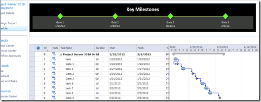

Anyway, lets get on with this post.

Step 1: Prepare to create the Milestone in Excel

• Navigate to the Business Intelligence Center of PWA, and to the Templates folder.
• Select the Projects and Tasks Template

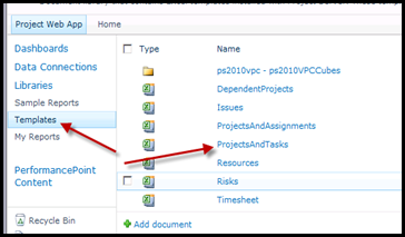
Once the template opens in Excel for Editing, navigate to the data connection properties as shown below.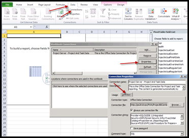

In the Command Text Section, replace the default query with

selecttaskname,taskstartdate,taskduration,taskismilestone,CAST(MSP_EpmTask_UserView.ProjectUID AS nvarchar(100)) AS ProjUIDfromdbo.MSP_EpmTask_UserView

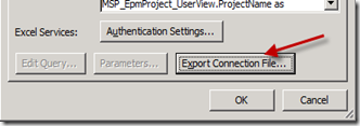
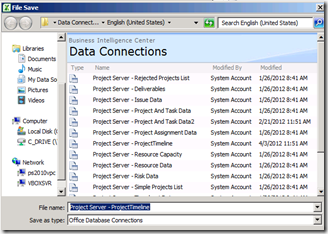
Click on Export Connection file, before you hit OK, and save the ODC with a different name, so that you are not overwriting the default template.

Once you do that, you will have the fields that you need to to build your Milestone View.

Step 2: Prepare to create the Timeline in Excel

Once you have the fields, it is a matter of building the right chart in Excel.

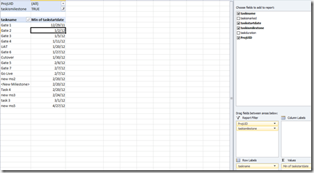
So, to start with, build the Excel Pivot Table, as shown below.

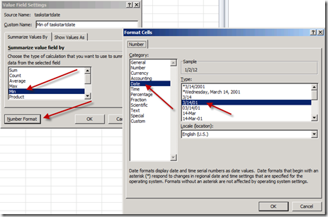
For the Values, when you insert the “Start Date” field, it will default to the “Count” of the Start date. We need to make sure that the “Min” of start date is displayed, and the number format is selected as Date.

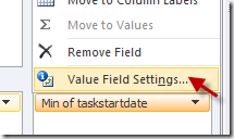
This can be achieved by clicking on the arrow besides the Start Date value, and changing it to Min and also changing the Number format as shown below.

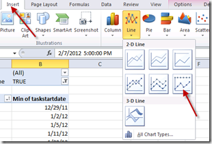
Now click on Insert Chart, and select the 100% stacked line with Markers Chart Type

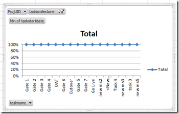
This will insert the Chart as shown below.

The easiest way I found to clean this up was to delete every item on the chart except the line with markers on it. which will leave you with something like this below.

Now beautify this  by adding Data Labels, color coding the Markers, changing the Marker Shapes and so on. After playing around with this a little, I arrived with the following format.

So now we have the Excel Milestone view created. It’s time to prepare and publish this to Excel Services.

That will be my next post….

Note: (A commercial Web part with additional features is available here, if you are interested in an off-the-shelf solution)